|
In May 2002, physicist, computer scientist, and
entrepreneur Stephen Wolfram unleashed his magnum
opus, a tome of 1197 pages, bearing the
not-so-humble title A New Kind of Science
(henceforth, ANKOS). The present text is not a review of
the book (the reader may visit this site for a collection of more
reviews of ANKOS one could possibly read) but a critique
of one of the fundamental pillars of Wolfram's
"theory of everything": his so-called Principle
of Computational Equivalence (henceforth, PCE), a
principle that, according to Wolfram,
What would be the worth of ANKOS should some claims that accompany the PCE shown to be wrong? In my view, the PCE would be reduced to an already known thesis, and the book itself would be nothing more than an interesting collection of types of cellular automata and other engines, a rather shameless collection of results already known by others and appropriated by the author of ANKOS, and a prime example of what kind of style should be avoided in prose, as it makes the reading of the text extremely difficult (there are repetitive syntactic patterns that appear from beginning to end ad nauseam, and the true content of the book can probably be expressed by one tenth of its volume, should normal, non-repetitive language be employed). |
What is Wolfram's Principle?
The Principle (of Computational Equivalence, or PCE) has not
been formally expressed in ANKOS; that is, there are no formulas
to describe it, only Wolfram's words. This is not without
precedent, however, since a very well-known (and related) thesis
in computer science, namely, the Church-Turing thesis, can only
be stated in words ![]() for example, in plain English. So let us grant Wolfram the same
inexpressibility of his PCE in formal terms, and see what it
states through Wolfram's own writings. In chapter 12 of ANKOS we
read:
for example, in plain English. So let us grant Wolfram the same
inexpressibility of his PCE in formal terms, and see what it
states through Wolfram's own writings. In chapter 12 of ANKOS we
read:
There are various ways to state the Principle of Computational Equivalence, but probably the most general is just to say that almost all processes that are not obviously simple can be viewed as computations of equivalent sophistication (ANKOS, pp. 716-717).
What does this cryptic sentence mean? To understand what Wolfram means with the above, we need to make a very short review of the first three chapters of ANKOS. I guarantee the review will be just short enough so that the reader who is already familiar with it will not be bored, but also sufficient enough to explain what ideas cropped up in Wolfram's mind.
In the first three chapters, the author of ANKOS introduces a
set of 256 cellular automata, which are very simple
"machines" that work in a pre-determined manner (like
most machines do), and yet produce visually interesting displays![]() at least a few of them do.
I put the word "machine" in quotes because these are
normally not mechanical devices with cogs and gears (although
there is no reason why they couldn't be), but pieces of software
that can be run on computer screens, including the page that you
currently read. Each such machine, called a rule by
Wolfram, has an incremental number between 0 and 255, which is
its name. Most rules, such as 0-17, 31-44, 46-59, and many
others, are utterly boring: they produce repetitive displays.
Once you have seen a few lines of them, you've seen them all.
Wolfram calls these "Class 1 rules".
at least a few of them do.
I put the word "machine" in quotes because these are
normally not mechanical devices with cogs and gears (although
there is no reason why they couldn't be), but pieces of software
that can be run on computer screens, including the page that you
currently read. Each such machine, called a rule by
Wolfram, has an incremental number between 0 and 255, which is
its name. Most rules, such as 0-17, 31-44, 46-59, and many
others, are utterly boring: they produce repetitive displays.
Once you have seen a few lines of them, you've seen them all.
Wolfram calls these "Class 1 rules".
| Rule 28 | Rule 54 | Rule 62 |
Figure 1: Outputs of a few of the Class 1 rules
Other rules, such as 18, 22, 26, 60, and a few more, show recursively repetitive behavior, where some pattern (usually a triangle) is repeated at various ever-increasing sizes. These are the "Class 2 rules".
| Rule 18 | Rule 150 | Rule 182 |
Figure 2: Outputs of a few of the Class 2 rules
Then we have "Class 3 rules", producing random patterns, at least in some part of their output.
| Rule 30 | Rule 45 | Rule 135 |
Figure 3: Outputs of a few of the Class 3 rules
Finally there are the "Class 4 rules", which play a special role in Wolfram's PCE. The rules of this last class produce output which is a mixture of randomness and patterned behavior. The prime example that figures prominently in ANKOS is rule 110.
Figure 4: rule 110 (Class 4)
Wolfram identifies only a handful of such rules, besides 110, that seem to belong to Class 4. Now, what's so special about rules in Class 4?
In chapter 11 of ANKOS it is hinted(1)
that rule 110 can be used to emulate a universal machine,
that is, a machine capable of computing any computable
function. Universal machines are known since the 1930's, and play
a very important role in theoretical computer science. Partly,
their importance is derived from the fact that any modern
computer, including the one you use now to read this page, has no
more computing abilities than a humble universal machine, in the
sense that there is no function your computer can compute that
can't also be computed by a universal machine. (In fact, the
opposite is true: there are some exotic functions![]() of theoretical interest
only
of theoretical interest
only![]() that can be
computed by a universal machine but not by your computer.) One
reason we use our familiar computers today, rather than universal
machines, is that the former are whole orders of magnitude faster
than the latter, in which we can't expect to implement any practical and useful
application, such as Microsoft Word, Adobe Photoshop, or
CMMS software. (CMMS software is used for maintenance activities of facility
equipment.). The
other part of the importance of universal machines lies in the
so-called Church-Turing thesis, which says that no
matter how hard we try, we can not hope to construct a device
computationally more powerful(2) than a universal machine.
Indirectly, this thesis has important theoretical implications
for human cognition, because if we assume that the human
brain is a device consisting of parts (neurons) that can be
simulated computationally by our familiar mathematical functions,
and if it contains no "magic" (no immaterial
parts that do not abide by the laws of physics), then it
follows from the Church-Turing thesis that the human brain, too
(hence, the human mind), can be simulated by a humble universal
machine (even though it would take entire centuries for such a
machine to do the simplest task that the human mind performs
effortlessly).
that can be
computed by a universal machine but not by your computer.) One
reason we use our familiar computers today, rather than universal
machines, is that the former are whole orders of magnitude faster
than the latter, in which we can't expect to implement any practical and useful
application, such as Microsoft Word, Adobe Photoshop, or
CMMS software. (CMMS software is used for maintenance activities of facility
equipment.). The
other part of the importance of universal machines lies in the
so-called Church-Turing thesis, which says that no
matter how hard we try, we can not hope to construct a device
computationally more powerful(2) than a universal machine.
Indirectly, this thesis has important theoretical implications
for human cognition, because if we assume that the human
brain is a device consisting of parts (neurons) that can be
simulated computationally by our familiar mathematical functions,
and if it contains no "magic" (no immaterial
parts that do not abide by the laws of physics), then it
follows from the Church-Turing thesis that the human brain, too
(hence, the human mind), can be simulated by a humble universal
machine (even though it would take entire centuries for such a
machine to do the simplest task that the human mind performs
effortlessly).
Now, universal machines were known long time ago; in particular, since the father of computer science, British mathematician Alan Turing showed that the so-called Turing machines can be turned into universal machines, with some clever programming. Also, various other devices have been shown to be capable of universal computation. Your computer, for example, loaded with some of its usual software (even a version of Microsoft's Excel suffices), is a universal machine to a very close approximatrion. So what's new with Wolfram's discovery that rule 110 can be also turned into a universal machine? Wolfram's intuition goes as follows:
Until now, we knew of universal machines as very specially crafted devices, with so many special-purpose parts that one would not expect to encounter them in nature, just by chance. But look! I propose to you my rule 110, which is so simple that one could expect to encounter it in nature, just out of mere chance! In fact, I've shown you in ANKOS that there are natural systems that seem to behave like the rules of some cellular automata (e.g., see the surface of some mollusk shells, ANKOS p. 423, and compare them with the output of some rules on the next page). If such a simple rule can be turned into a universal machine, then we should expect to find universal machines much more often than we thought in nature!
These are not the exact words Wolfram uses, but the gist of hundreds of pages of his book.
So what? ![]() one
might ask
one
might ask![]() What's the
deal if universal machines can be more common than we thought, in
nature?
What's the
deal if universal machines can be more common than we thought, in
nature?
Well, that observation has important implications regarding intelligence. If human brains can be seen as universal computing devices, and if universal computers are common in nature, this means that intelligence, too, is common in nature. We may expect to encounter intelligence in other star systems more often than we previously thought. Don't you agree that this is important? In a lecture I gave at Indiana University, in Bloomington, Indiana, on April 7, 2003, I claimed that just like the Copernican revolution placed the Earth away from the center of the universe, and just like Darwinian evolution placed human beings away from a supposed special role in nature, similarly, the revolutionary ideas that I propose place intelligence away from a privileged and unique position in cosmic matters. (These were not my exact words, but the lecture has been videotaped and is available for anyone who cares to see it.)
Hold it!![]() the
skeptical listener might retort
the
skeptical listener might retort![]() Just because rule 110 is simple doesn't mean that we
can find devices implementing rule 110 in nature!
Just because rule 110 is simple doesn't mean that we
can find devices implementing rule 110 in nature!
But this is what the Principle of Computational Equivalence is about!
Wolfram might answer
But... but... every simple machine is not implementing a universal computer! It needs a program to do so. And, as you show in chapter 11 of ANKOS, it takes an extremely complicated program to turn a device, such as rule 110, into a universal computer. The same can be said for every computing device. A Turing machine can be quite simple in its machinery (although not as simple as rule 110), but it takes a very complicated program to turn it into a universal computer, one that is actually capable of simulating every other Turing machine. Do you mean that because of the PCE we should expect to find those simple devices together with their intricate programs (that turn them into universal computers) in nature? Wouldn't that be like encountering William Paley's famous watch(3) on the sandy beach of a deserted island? Wouldn't the program itself imply purposeful and intelligent design?
No. You don't need to expect to encounter the program. A device, such as rule 110, is sufficient. If you read chapter 12 of ANKOS carefully, you'll see that the idea is that you can get arbitrarily complex behavior from practically every input. That is, any initial program (input) will do. Please, do read what I wrote in chapter 12:
"But the Principle of Computational Equivalence asserts that in fact even if it comes from simple initial conditions almost all behavior that is not obviously simple will in the end correspond to computations of equivalent sophistication" (p. 724).
"Quite often part of the reason for this [...] is that even with a single very simple initial condition the actual evolution of a system will generate blocks that correspond to essentially all possible initial conditions. And this means that whatever behavior would be seen with a given overall initial condition, that same behavior will also be seen at appropriate places in the single pattern generated from a specific initial condition" (p. 724, underlining added).
Let us interrupt here this virtual dialog and see what Wolfram means with the above excerpts from ANKOS.
He says this: you don't need an intricate and carefully designed initial program (he calls it "initial condition") to your rule 110 (or any "equivalent" device, in the PCE sense) to arrive at a universal computer. Any odd input will do! The reason is that you may start with simple (say, random and short) input, but the rule will generate very complex behavior out of that. All you need to do is look sufficiently far down in the output produced by your automaton, and due to the complexity of the output and the fact that it can be run indefinitely, you are guaranteed to find your carefully designed program, with all its computation, as a sub-block in the overall block of the output!
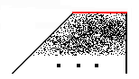
Let's draw some diagrams to understand this. Suppose our intricate initial program for rule 110 that performs some meaningful computation is the following red line:
![]()
Figure 5: Initial program
That is, imagine we take a bird's eye view and we see this program from very far, when in reality it consists of thousands of bits that we can only discern if we take a close-up look. This may even be the program that turns rule 110 into a universal computer (that is, the "proof" hinted at in chapter 11 of ANKOS), but it doesn't have to; it can be any computation, for example, the function that computes the logarithm of a number. Notice that I assume this program is finite, since only finite objects may appear in nature, and we are interested in the possibility of natural occurrences of rule 110. So, if we give this program as input to rule 110, we'll get the usual trapezoidal output that this rule always produces (see Theorem 1, below, for a simple proof of that), which will be the running of some particular computer (a function) with some particular input. The output of our initial program is shown schematically on the next figure.
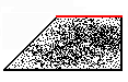
Figure 6: Output of the program
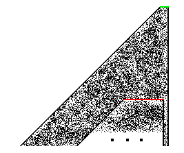
The argument of our previous skeptical interlocutor was that
we can't expect to encounter such an intricate computation![]() the entire trapezoid
the entire trapezoid![]() by chance in nature.
(Remember, the red line stands for thousands of individual bits.)
Wolfram's reply is that you don't need to expect to find the
above trapezoidal entity from the very start. All you expect to
see nature do is feed the device with some random input, and the
complexity of the output (together with the fact that it extends
indefinitely) guarantees that you will encounter the trapezoid of
the previous figure as a sub-block in your overall output, as
shown in the next figure:
by chance in nature.
(Remember, the red line stands for thousands of individual bits.)
Wolfram's reply is that you don't need to expect to find the
above trapezoidal entity from the very start. All you expect to
see nature do is feed the device with some random input, and the
complexity of the output (together with the fact that it extends
indefinitely) guarantees that you will encounter the trapezoid of
the previous figure as a sub-block in your overall output, as
shown in the next figure:
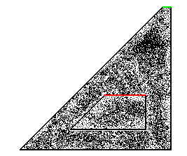
Figure 7: The program as a sub-block of random output
Here, the short green line on top represents the random
initial input (what Wolfram calls the "single very
simple initial condition" in the excerpt,
above). You give your random input, let the rule run
sufficiently long, and, presto!![]() you get your wanted sub-block somewhere further down
in the output. That's what "the actual evolution of a
system will generate blocks that correspond to essentially all
possible initial conditions" means (same excerpt, see
above).
you get your wanted sub-block somewhere further down
in the output. That's what "the actual evolution of a
system will generate blocks that correspond to essentially all
possible initial conditions" means (same excerpt, see
above).
We will soon proceed to show that Wolfram's PCE is false: contrary to his claim, we don't get a sub-block with the sought-for computation anywhere in the overall output of rule 110 if we start with random input. But before we see why we don't, let us examine the consequence of this refutation: what would it mean to show that rule 110 does not spontaneously result in universal computation?
Wolfram uses rule 110 as his prime example of a candidate for "automatic" (spontaneous) universal computation. If rule 110 doesn't do the job, one wonders which cellular automaton would do it. Wolfram's PCE becomes then a statement the content of which is already known. It simply reduces to this: there are some cellular automata capable of universal computation, but under very special initial conditions. However, we already know that. It has been shown that one can construct a (very intricate) input in the well-known Game of Life (probably the best explored case of a two-dimensional cellular automaton) that acts as a Turing machine (designed by Paul Rendell, in 2000). It is a special-purpose Turing machine, not a universal one, but given the construction I do not think anyone seriously believes that the design of a true universal Turing machine in the Game of Life is impossible. This shows that an automaton as simple as the Game of Life already possesses the ability for universal computation. The problem for PCE is that such designs are extremely complicated, brittle (usually flipping the value of any single bit results in chaos), and hand-crafted, which means that we don't expect to find them in nature. I conclude from all this that Wolfram's "discovery" about rule 110 is neither exceptional nor terribly interesting, and certainly not one that can be elevated to the status of a natural principle, especially one that "has vastly richer implications [...] than essentially any single collection of laws in science." (p. 726)
In particular, what will be demonstrated is that the trapezoid shown schematically in figure 6, (the sought-for "computation") cannot be found as a sub-block as shown in figure 7 in the vast majority of cases. It cannot be proven that it can never be found, because, after all, if the proof of the universality of rule 110 is correct, there must exist some extremely rare (and long!) initial inputs that manage to produce the sought-for trapezoid of figure 6. But Wolfram doesn't claim that. As we saw, he claims that any random initial input will in the end produce the sought-for trapezoid. I will show that one needs to be extremely lucky for that to happen. Therefore, what follows is not a proof, in the mathematical sense, but a probabilistic argument. Wolfram's claim is also a probabilistic one, betting on the high probability with which his claim should be satisfied. It will be shown below that the probability for his claim to be satisfied is practically zero.
First, let us agree on what the trapezoid of figure 6
represents: it represents a computation. One enters the
initial input (the red line), allows the rule to do its job
(i.e., the bits are manipulated according to the rule), and after
a while, if the computation terminates (we'll soon see
what this means), we get the final line that defines the base of
the trapezoid and![]() for
us
for
us![]() the end of the
computation. How exactly we read the result of this computation
does not need concern us here. We may read the last line and
interpret the bits in some particular way, or we may look at the
patterns that "survive" in the very last rows; but it
really doesn't matter how we interpret the result for the
discussion that follows. All that matters is that every trapezoid
corresponds to some computation.
the end of the
computation. How exactly we read the result of this computation
does not need concern us here. We may read the last line and
interpret the bits in some particular way, or we may look at the
patterns that "survive" in the very last rows; but it
really doesn't matter how we interpret the result for the
discussion that follows. All that matters is that every trapezoid
corresponds to some computation.
What we haven't established yet is that rule 110 produces only trapezoids like the ones in our figures. Let's prove this, first.
Theorem 1: Rule 110 results in trapezoids, with their left side slanted by 45 degrees, and their right side exactly vertical.
Proof: The initial input has to have a leftmost black bit, and a rightmost black bit, since it is assumed to be finite. To see that these two bits on the two edges of the input are going to create the lines described by the theorem (slanted at 45o on the left, vertical on the right), we need to examine what the definition of rule 110 is. The rule can be described schematically as follows (see also ANKOS p. 32):
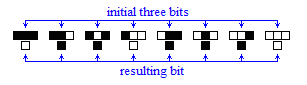
Figure 8: The definition of rule 110
The black and white bits in figure 8 show how the resulting
bit is computed, given its three prior ("neighboring")
bits, just above it. For example, if all three prior bits are
black, then the resulting bit is white (first T-like object, on
the left); if they are like black-black-white, then the resulting
bit is black (second T); and so on. Now it's easy to see why the
leftmost side of the trapezoid will be slanted by 45 degrees. To
have the first black bit on the left (looking at the input from
left to right), we need all bits to the left of this black bit to
be white. The only T-objects that match this prescription in
figure 8 (that is, first, one or more white bits, then a black
bit, and then anything) are the fifth, sixth, and seventh T. The
fifth and sixth result in extending the leftmost bit directly
downwards, while the seventh T is the one responsible for
extending it down-and-left, at a 45 degree angle. None of these
three T's results in moving the leftmost bit to the right. Also,
when we look at the leftmost bit, the two bits on its left have
to be white, hence the T-object that will apply first is the
seventh one; therefore there will be an immediate extension of
the leftmost bit in the down-and-left direction. This shows that
a slanted (at 45 degrees) leftmost line will be created. Now, for
the rightmost vertical side, the reasoning is similar. To have
the first black bit on the right of the input (now looking at the
input from right to left), we need all bits to the right of this
rightmost black bit to be white. The only T-objects that match
this prescription in figure 8 (that is, one or more white bits on
the right, then a black bit, and then anything) are the second,
fourth, and sixth. Of these, the fourth one shows what happens
when we encounter the rightmost bit: the resulting bit remains
white, directly under the "middle" white bit. None of
these three T's moves the rightmost black bit either to the right
or to the left; the only thing that can happen is that the bit
can be propagated directly downwards. Hence, once we encounter
the rightmost black bit, a vertical black line will be formed
downwards, which is the vertical right side of the trapezoid.
This concludes the proof of our theorem. ![]()
The phrase "if the computation terminates", in a prior paragraph, is important. If the initial input in figure 5 represents any computation, this means that we cannot be talking about a single input (a single red line), but about an infinity of inputs (an infinite number of red lines). The reason is that the set of all computations is infinite. Likewise, the set of all trapezoids that are expected to be observed as sub-blocks from random input in rule 110, is also infinite.
Now the important observation is that some of these trapezoids will have to be infinite in height. This must be the case because rule 110 is supposed to be universal. Hence, the red-line trapezoids compute every computable function. It is known in theoretical computer science that not all computations terminate. In fact, the set of those computations that do terminate is called the set of "total recursive functions", and we don't need a lot of computing machinery to evaluate them: even the most restricted set of machines, known as "deterministic finite automata" (less powerful than Turing machines, or rule 110), can do the job. What such a finite automaton cannot perform is one of those computations that never end: for those, we need the power of a Turing machine, or of rule 110 (or any other equivalent device, such as your computer). Thus, the set of all computable functions, including those that result in a potentially infinite computation, is called "recursively enumerable functions" (r.e. functions). These are the functions that rule 110 must be able to handle if it is to be conferred the title of a machine with the potential for "universal computation". Therefore, some of the trapezoids (some of those that compute r.e. functions but not total recursive ones) extend infinitely downwards: they are bottomless. This observation necessitates a re-drawing of figure 6, as follows:
Figure 9: An infinite computation
The three dots and the lack of a bottom line in the above trapezoid represent the fact that this is a non-terminating(4) computation. Wolfram's claim implies that we should encounter as sub-blocks of any computation (with random input) not only the finite trapezoids, but also the infinite ones; otherwise, if there are some trapezoids that never appear as sub-blocks, Wolfram's claim becomes void of content, because rule 110 turns out to be incapable of producing all computations, contrary to a genuine universal machine. (In other words, if only finite trapezoids are to be found, rule 110 would spontaneously compute only the set of total recursive functions.) With the knowledge that we have to accomodate such infinite trapezoids as sub-blocks the previous figure 7 needs to be redrawn. Let us see how such trapezoids can be placed within the overall output.
Figure 10: Two possibilities for placing the infinite sub-block within the larger trapezoid
Figure 10 shows two possibilities for the placement of the
infinite computation within the overall (also infinite)
trapezoidal output. Although the right-hand drawing of figure 10
is a special case of the drawing on the left, I strongly
suspect(5)
that Wolfram has the right-hand drawing in mind when he talks
about the computation appearing spontaneously![]() that's why I prefer to draw this case
explicitly. Whatever the placement of the smaller trapezoid
within the larger is, I proceed now to show that no such case
will appear in practice, except probably under extremely rare
conditions with carefully designed initial inputs (top green
lines).
that's why I prefer to draw this case
explicitly. Whatever the placement of the smaller trapezoid
within the larger is, I proceed now to show that no such case
will appear in practice, except probably under extremely rare
conditions with carefully designed initial inputs (top green
lines).
To see why this is so, we need to make a number of observations regarding rule 110. The most important of these observations concerns the "duration of activity" in this rule. Let me explain what I mean by that.
If we pay close attention to the output produced from random input by rule 110, we'll notice the creation of a ubiquitous "background pattern" (consisting of tiny 3x3 triangles), against which different patterns seem to be "running down", as time advances downwards. We'll call these running pattern "gliders", as is the customary term in cellular automata of this type. The following figure shows what is meant by these terms.
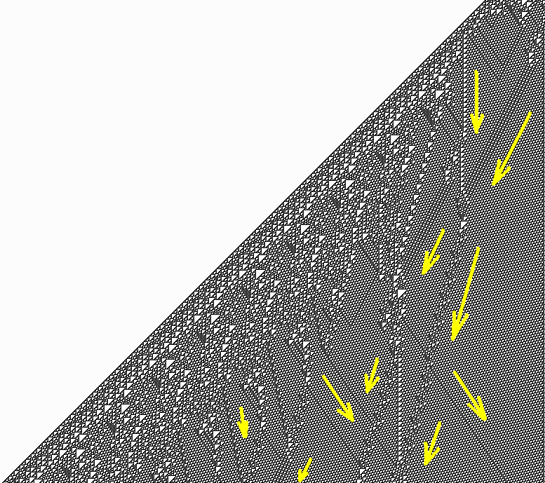
Figure 11: Typical output from rule 110 with some "gliders" highlighted
Some of the spontaneously generated gliders have been marked with yellow arrows running in parallel with them in figure 11. Such gliders are the "gears" of meaningful computations in rule 110. What happens is that sometimes these gliders crash against each other as they move downwards in converging straight-line paths, and often different gliders shot at different angles are produced by the collision; the new gliders then crash against other pre-existing ones, and so on. Thus, a flurry of activity seems to be happening for a while, and we can imagine that "information" is exchanged between gliders through their collisions. If the initial input is designed carefully (down to the last bit), then it is possible (or at least imaginable) to produce a meaningful computation in which, after information has flown from glider to glider in a pre-determined way, and after gliders have been generated and extinguished for awhile, we end up with a specific pattern of gliders, at which point we announce the "end of computation" (although the rule may keep running indefinitely, of course), and interpret the resulting surviving gliders in order to read out the result. For example, the interpretation may be that if such-and-such gliders are present (or absent) in the few most-recent lines, then the current stream of bits in the output represents the answer "YES, number 1777 is a prime number" (assuming this was the question our automaton was attempting to answer). The discussion that follows is independent of what exactly our convention for reading the output is.
How far down in the output can the spontaneous activity of gliders continue? It is my intention to convince the reader that what happens in nearly every case of initial input is this: some gliders keep interacting for awhile, depending on how many they were to begin with, but after some number of time-steps (which is usually not too large compared to the number of the initial input bits) the behavior of the gliders becomes predictable. What I mean by this is that the remaining gliders keep moving at either diverging or parallel directions, so that they never meet again (see figure 12). No glider can run at an angle less than 45o with the horizontal direction (in fact, the limit seems to be higher), so that none of them interferes with the left slanted margin (which forms an angle of exactly 45o with the horizontal direction). Those gliders that crash against the vertical right border are either "absorbed" by it (disappear) or "bounce", creating other gliders that sooner or later end their interactions with the rest. After awhile, a "bird's-eye view" reveals the following picture:
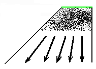
Figure 12: The situation after glider activity has ceased
What we see schematically in figure 12 is a number of gliders that diverge, and are never going to meet, either among themselves, or with the borders. Once we know their patterns at a certain time (the base of the arrows in the figure) and the angle at which they move, their further evolution is completely predictable; which means we can predict the state of the output for any value of time, no matter how large, and we can make our calculations in finite (and short!) time. It's like knowing where the planets of our solar system will be at any time in the future, simply by having the equations of their orbits and knowing their current state of motion (even better, in fact, because in our case we can issue predictions with exactly 100% certainty, while in the case of planets it can be hypothesized that our knowledge of their laws of motion is not 100% accurate). We have not yet been convinced that the situation shown in figure 12 is a typical one. We'll come to the conviction-point soon; but before we do so, let us take a preview:
Where does all this lead to? Simple: I want to argue that a
computation such as the one shown schematically in figure 12 can
never compute a class of functions that every "universal
computer" must be able to compute. What do such functions
look like? What is their characteristic, why are they
incompatible with figure 12? Well, basically they progress in
such a way so that we cannot predict their behavior beforehand.
Take, for example, a computation that attempts to prove a theorem
given a number of axioms (in other words, an automated
theorem prover). It is well-known in the theory of
computability that such a function is semi-decidable: if
the theorem can be proved, then the theorem prover will stop at
some point and output YES (it may also print the proof, but that
is secondary in importance; what's primary is that the
computation will terminate). If, however, the theorem cannot be
proved from the given axioms![]() and we cannot know this in advance
and we cannot know this in advance![]() then the machine will
continue trying, and trying, and will continue to try forever,
but as long as we watch it we don't know if it will indeed go on
working forever or it will stop at some point and answer YES
(except in some uninteresting cases with trivial sets of axioms).
That's what is semi-decidable: if there is a proof, the
machine answers YES; if there isn't one, the machine never
answers.
then the machine will
continue trying, and trying, and will continue to try forever,
but as long as we watch it we don't know if it will indeed go on
working forever or it will stop at some point and answer YES
(except in some uninteresting cases with trivial sets of axioms).
That's what is semi-decidable: if there is a proof, the
machine answers YES; if there isn't one, the machine never
answers.
Imagine now that the machine shown in figure 12 is
such a theorem prover, and it's trying to prove a theorem. I will
show in a moment that this cannot be the case, because being in a
position to predict the future output of a machine like the one
in figure 12 (to infinity!) we would be in a position to detect
whether the word YES will appear in its output or not.
That is, we would be in a position to answer with absolute
certainty that the word YES does not appear in the
output, if such is the case; but this cannot be true for a
semi-decidable theorem proving computation, because if it were,
we would be able to know that the machine will never
prove the given theorem. That would turn theorem-proving to a
completely decidable problem![]() which we know is false.
which we know is false.
Let us now put the pieces together.
First, the claim was made that figure 12 depicts a typical situation. Is this true? Do we get a flurry of activity with gliders for some finite time starting with random input, until all interesting interactions among gliders dwindle and cease, and we end up with a bunch of gliders (or none at all) that move downwards and to the left, either in parallel directions, or diverging from each other?
Such questions are usually very difficult to answer with
absolute certainty in the domain of cellular automata. In this
domain (which is a sub-domain of the theory of complexity) often
there is no better way to answer a question other than running
the system and noticing its behavior. In other words, it can even
be proven![]() in
some cases, at least, not necessarily in the questions that
concern us here
in
some cases, at least, not necessarily in the questions that
concern us here![]() that there
is no proof answering a question, no shortcut, no predictive
method to tell us the answer, other than letting the system do
the computation according to its rules and letting us observe
what the end result is. Such
computations, for which we cannot give a predictive answer before
they run, are said to be incompressible.(6)
Classical mathematical theory-making, of the genre proceeding in
the theorem-proof fashion, is of no avail in such cases.
that there
is no proof answering a question, no shortcut, no predictive
method to tell us the answer, other than letting the system do
the computation according to its rules and letting us observe
what the end result is. Such
computations, for which we cannot give a predictive answer before
they run, are said to be incompressible.(6)
Classical mathematical theory-making, of the genre proceeding in
the theorem-proof fashion, is of no avail in such cases.
I cannot be sure that a theorem answering the above questions with its proof does not exist, and it seems very hard for me to come up with such a proof. Consequently, I plan to convince the reader by bringing evidence that glider activity ceases and their motion becomes predictable after awhile in the vast majority of cases.
Categorema:(7) In rule 110, the vast majority of computations that start with random input result in a finite initial part where gliders interact unpredictably, and an infinite final part where gliders do not interact with each other, and their future state in space and time is completely predictable.
Evidence:(7)
The best way I can bring evidence to support the above claim is
by designing a realistic situation with some initial random
input. The following figure is an interactive one. The reader may
specify the initial input bits either manually (clicking on the
top-right row of boxes) or automatically (clicking on button ![]() , which
assigns random values) and then run the rule by clicking on the
button with the running figure:
, which
assigns random values) and then run the rule by clicking on the
button with the running figure: ![]() . Buttons
. Buttons ![]()
![]()
![]() and
and ![]() as well as the scrollbars, can
be used to scroll in the corresponding directions and watch
further portions of the output. The last-generated and current
epoch (time) under the mouse pointer are displayed on the status
bar, at bottom. (Notice that the very first line
as well as the scrollbars, can
be used to scroll in the corresponding directions and watch
further portions of the output. The last-generated and current
epoch (time) under the mouse pointer are displayed on the status
bar, at bottom. (Notice that the very first line ![]() the initial input defined
by the top-right row of boxes
the initial input defined
by the top-right row of boxes![]() is omitted; the output proceeds from the second line
is omitted; the output proceeds from the second line ![]() epoch #1
epoch #1 ![]() onward.)
onward.)
Figure 13: Interactive display for amassing evidence in support of the present categorema
The above interactive figure shows the output of some random computation. What I observe is this: some gliders are generated very soon, start interfering with each other, crash, generate a few more gliders... and that's all. After a while we end up with a completely predictable set of gliders that, as in figure 12, either diverge or are parallel, and in any case do not interact with each other or with the trapezoid's borders.
Is this situation an outcome of the specific initial bits that I chose? The reader may experiment by choosing different initial input (bits), varying their number, too. I repeated many times this experiment and gathered some statistics, which I present here. The statistics link the length of the initial input with the finite height of the area of unpredictable activity (what is depicted as a fuzzy collection of bits in figure 12). In all trials I observed a finite height for the unpredictable area. However, the population of trials has three distinct peaks in its distribution, as a result of three different patterns forming on the left (slanted) border. The following figure shows these three different patterns.
| Pattern #1: | 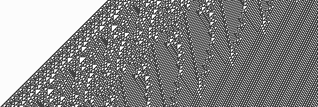 |
| Pattern #2: | 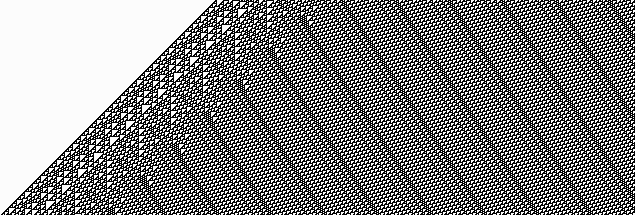 |
| Pattern #3: | 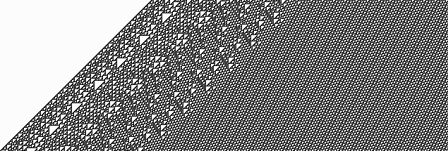 |
Figure 14: The three patterns at the left border of rule 110
What I refer to as "patterns", above, is the pattern
of parallel lines that appear on the right side of each of the
three cases in figure 14, but actually are on the left side of
the overall trapezoidal output (the above three trapezoids are
excerpts at random positions of the left sides of three different
input cases). Each of the three patterns is formed at random,
with the first being the most common, the second a bit more rare,
and the third very rare. Depending on which pattern is formed,
the distribution of the random function "length of input
versus height of unpredictable area" is different.
I experimented with three different input lengths: 100, 200, and
300 initial input bits, and I repeatedly ran the rule until I
gathered 30 observations with pattern #2 in each case. This means
that, as a consequence of the pattern frequences, I gathered a
few more observations for pattern #1, and a very small number for
pattern #3 (for which I do not care ![]() we'll soon see why). Here is the
statistics through which my observations can be summarized:
we'll soon see why). Here is the
statistics through which my observations can be summarized:
|
|
|
||||||||||||||||||||||||||||||||||||||||||||||||||||||||||||
What I conclude from the above data is the following:
In pattern #1, which is the most frequently ocurring, for an initial input length of 100 bits we get an average height of unpredictability of 1547. This means that the gliders keep interacting with each other unpredictably for an average of 1547 epochs (time-steps, "downwards"), before they produce predictable straight lines, as in figure 12. The last line in this table tells us that with a confidence of 99% we can be sure that the average height does not exceed 2416 epochs. These numbers increase slightly as we increase the initial input length, but not much.
A similar observation holds for pattern #2, except that here the mean heights of unpredictability are somewhat larger than the corresponding numbers of pattern #1, but the smaller number of observations (30) allows some margin for error. I believe that the mean height of unpredictability actually keeps increasing with the length of the input for pattern #2, too, given a sufficiently large number of observations.
Finally, pattern #3 can be ignored altogether: its mean heights seem to yield smaller numbers than the other two patterns, and its frequency of occurrence seems to be decreasing when the length of the input is increasing. If this is true, pattern #3 statistically does not play a significant role. Notice that its last column gives a large number for the 99% confidence limit because there were only two observations, one of which yielded a high value (17883 epochs), resulting in a large standard deviation. With two observations only, that number (31562) is statistically insignificant.
My overall conclusion from these observations is the
following: the mean height of unpredictability seems to be a
number at most one order of magnitude larger than the initial
input length, and seems to increase rather linearly with the
input length (if not sub-linearly). It is bounded with a high
confidence by numbers that are of the same order of magnitude
(less than twice as large). Probably the most important
observation for our categorema is that out of a total number of
236 observations (37+41+53+3*30+7+6+2), all resulted in a finite
region of unpredictability, and an infinite region of
predictability, which concludes the evidence for our categorema. ![]()
So, the categorema claims that the "interesting" part of the computation is finite, that is, the part that can "surprise" the observer, ends sooner or later (rather "sooner", I'd think, judging from the statistics, above). Following that finite part is an infinite ocean of predictability and, hence, boredom. What I want to finally show is that in an ocean of boredom we can always tell whether a certain pattern (meant to be the "answer" of a computation) exists or not. For example, if the answer is "YES", we do not need to search the infinite ocean bit by bit (a search that would never end), but we can do our calculations and predict whether the pattern is going to appear somewhere in the ocean or not, without being forced to let the rule run and sit back and watch. In the theorem that follows, the phrase "a pattern of bits" refers to something like an encoding of an answer, such as "YES", in structures (e.g., gliders) provided by an automaton such as rule 110.
Theorem 2: If the output of rule 110 consists of an ultimately predictable (i.e., predictable to infinity beyond some time-step) list of gliders that do not interact with each other (i.e., they are either parallel or diverge, as in figure 12), then there is an algorithm that can tell us whether a given pattern of bits will be formed at some point in the output or not (i.e., the algorithm always terminates with a yes/no answer).
Proof: We proceed to prove the theorem by constructing the algorithm that gives us the answer.
The following figure is a near-repetition of figure 12, except that it shows a rectangular region, somewhere in the infinite predictable region of gliders, which is supposed to be the encoding of the pattern of bits (such as "YES") that we are looking for, in terms of gliders. In other words, the gliders together with the background form this pattern of bits that we are looking for.
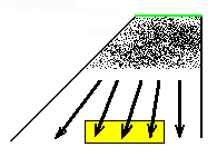
Figure 15: The highlighted rectangular region is the pattern of bits we are looking for
Here is how we can tell whether the pattern (the yellow box in figure 15) is ever going to be formed within the trapezoid or not. First, we assume the pattern is finite; otherwise there is no way it can fit within the output of rule 110, since by theorem 1 each horizontal line is finite. Since the pattern is finite, there is only a finite number of gliders that may participate in its formation. Let's denote by G the overall set of gliders that do not interact in this final infinite region (all the black arrows in Fig. 15). In the algorithm that follows, it is assumed that we can determine whether a given glider participates in the formation (is part of) of the pattern or not. This can be done with a finite search on the pattern (e.g., from left to right), since the given glider consists of a finite periodically repeating sequence of bits, and the pattern is also finite. We proceed as follows:
For each of the gliders gi in G do the following:
   Assign gi to g1 if it is the first (leftmost) glider participating in the formation of the pattern.
   Assign gi to g2 if it is the last (rightmost) glider participating in the formation of the pattern.
Now, having found g1 and g2 do the following.
If g1 and g2 are parallel, then
   All the rest of the gliders between g1 and g2 must also be parallel (i.e., all gliders
   participating in the pattern must have the same direction).
   This means that the interval between each two successive gliders is known (since
   they are all parallel, their mutual distance remains invariant).
   Hence it suffices to examine the gliders gj between g1 and g2 in sequence, and
   If all gj participate in the pattern, then
      Exit answering: "YES, pattern is formed"
   Else
      Exit answering: "NO, pattern is not formed"
Else g1 and g2 are not parallel; then
   g1 and g2 have to be diverging; hence there will be a single epoch t at which
   these two gliders attain a mutual distance which is exactly equal to the one
   that they exhibit in the pattern. (Epoch t can be easily calculated since we know
   how fast g1 and g2 diverge from each other, as well as their initial distance.)
   Examine the output of the rule at epoch t.
   If the pattern appears at t, then
      Exit answering: "YES, pattern is formed (at epoch t)"
   Else
      Exit answering: "NO, pattern is not formed"
(The indentation is supposed to show where each programming block starts and ends, thus avoiding explicit pairs of braces, or begin-end tokens.)
The above algorithm always terminates and answers either YES,
or NO, from one of its exit points, which concludes the proof.![]()
What the categorema and theorem 2 show is that, starting with random input, rule 110 may compute spontaneously only the total recursive functions. In other words, rule 110 spontaneously may be expected to have only the power of a deterministic finite automaton, not of a Turing Machine, let alone a Universal Turing Machine. Hence, it's not expected to result in universal computation. I emphasized the word may, previously, because frankly, I "strongly suspect" that rule 110 spontaneously computes nothing at all. That is, if we are willing to call a "computation" what we see coming out of random input, then the arrangement of molecules in a rock may be said to "compute", too; but then, the word "computation" loses its meaning, becoming all-inclusive, thus making it possible to apply it to practically every random arrangement of items in the world.
Where does all this discussion place rule 110 in the set of
computing devices? Assuming that rule 110 is capable of universal
computation, it should be placed at the far end of a spectrum of
"machines" (some of them theoretical, some of them very
real), all of which have the ability for universal computation,
but they differ in the amount of pre-existing "gear"
that they offer to the programmer in order to specify and execute
a computation. I'll explain. Most people are more familiar with
machines of the other end of the spectrum, opposite to rule 110,
such as Mathematica (Wolfram's own brainchild). In Mathematica,
if one wants to compute, say, the function x2 (the
square of a number), all one needs to do is type three
characters: x^2, hit shift-Enter, and, assuming
x has already been assigned a value, one gets the result
immediately on the next line. The minimal effort on the user's
part is possible because there is a huge amount of programmed
"gear" lurking in the background, all part of the
machinery provided by Mathematica for doing just this sort of
computations (and much more). Next to Mathematica in the range of
universal computing machines stand programming languages, such as
LISP (or any LISP-like language). In LISP one needs to type a few
more characters to get the result of x2, for example,
something like (times x x) and hit Enter. LISP's
engine is significantly less loaded with "gear" than
Mathematica's, is less oriented towards math functions and more
towards symbolic processing, and anticipates to a lesser degree
what the user might type![]() it is more general as a programming language, after
all. Next to LISP in this spectrum stand other programming
languages. As an example, in C++ (or plain old C) one needs to
type more characters if one wants to compute the square of a
number. So, something like: int square (int x) { return
x*x; } is necessary, and I omitted a "main"
entry that's mandatory for a program in C++ to compile and run
properly. That's because C++ has even less "computing
specialization" than LISP (although as an engine is probably
larger), is slightly more of a "general purpose
language", and expects the user to do even more work before
computing anything. One can move further down in this spectrum
with assembly language (particular to each type of computer, but
symbolic), machine language (particular and non-symbolic, just a
stream of machine instructions in bits), and even further with
various theoretical constructs, such as RAM machines, Turing
machines, and cellular automata. The latter can provide further
examples, such as the Game of Life (with constructions similar to
Paul Rendell's turning them into universal computers), and rule
110 (with Matthew Cook's proof). In each case, as we move down in
this spectrum, we need to enter longer and longer programs in
order to compute a simple function such as x2, while
the "bare bones" of the engine become progressively
simpler. With rule 110 occupying the last position in this
spectrum, we see that the bare bones become probably as simple as
they can be (you can see all of the engine in figure 8, above),
but the specification of the program in rule 110 for computing
the square of a number (of any number, not just, say,
four) must be extremely long (I don't know what it could be like
it is more general as a programming language, after
all. Next to LISP in this spectrum stand other programming
languages. As an example, in C++ (or plain old C) one needs to
type more characters if one wants to compute the square of a
number. So, something like: int square (int x) { return
x*x; } is necessary, and I omitted a "main"
entry that's mandatory for a program in C++ to compile and run
properly. That's because C++ has even less "computing
specialization" than LISP (although as an engine is probably
larger), is slightly more of a "general purpose
language", and expects the user to do even more work before
computing anything. One can move further down in this spectrum
with assembly language (particular to each type of computer, but
symbolic), machine language (particular and non-symbolic, just a
stream of machine instructions in bits), and even further with
various theoretical constructs, such as RAM machines, Turing
machines, and cellular automata. The latter can provide further
examples, such as the Game of Life (with constructions similar to
Paul Rendell's turning them into universal computers), and rule
110 (with Matthew Cook's proof). In each case, as we move down in
this spectrum, we need to enter longer and longer programs in
order to compute a simple function such as x2, while
the "bare bones" of the engine become progressively
simpler. With rule 110 occupying the last position in this
spectrum, we see that the bare bones become probably as simple as
they can be (you can see all of the engine in figure 8, above),
but the specification of the program in rule 110 for computing
the square of a number (of any number, not just, say,
four) must be extremely long (I don't know what it could be like![]() I'm just guessing). That's
what the characteristic of this spectrum of machines is: you lose
in "machine gear"
I'm just guessing). That's
what the characteristic of this spectrum of machines is: you lose
in "machine gear" ![]() the machine becomes skinnier
the machine becomes skinnier ![]() but you gain in program length: your
program becomes long and unwieldy. Rule 110 is nothing but an
occupant of one end of this spectrum. If this is true, it's an
interesting addition that should be attributed to Wolfram and
Cook. It is also interesting that Wolfram is responsible for both
ends of the above spectrum; but, I think, there is nothing deeply
profound in all that.
but you gain in program length: your
program becomes long and unwieldy. Rule 110 is nothing but an
occupant of one end of this spectrum. If this is true, it's an
interesting addition that should be attributed to Wolfram and
Cook. It is also interesting that Wolfram is responsible for both
ends of the above spectrum; but, I think, there is nothing deeply
profound in all that.
If rule 110 does not spontaneously result in universal computation, what is the implication of this observation for Wolfram's PCE?
As I mentioned earlier, Wolfram bases his "strong
suspicion" for the spontaneity of universal computation on
the behavior of automata such as rule 110, and explains this in
chapter 12 of ANKOS. Probably aware of the subtle difficulties, a
few pages later in the same chapter he starts referring to rule
30 (as exemplifying the idea of the appearance of sub-blocks
within the overall output of the rule), sweeping under the rug
the observation that rule 30 belongs to his Class 3, not Class 4,
which is the one that is supposed to consist of rule-outputs that
are neither random nor obviously simple. Thus, there is
essentially no supporting evidence for the spontaneity of
universal computation coming from any of his 256 1-dimensional
cellular automata. If there are different kinds of automata that
may support this thesis, the burden of proof is on Wolfram's
shoulders, not on the rest of the scientific community![]() because I do not suppose
Wolfram expects people to start examining different kinds of
cellular automata in an effort to validate his claims, just
because he strongly suspects that there are some automata that
support them. Besides, Wolfram talks about "every process
that is not obviously simple" being capable of universal
computation, not just some, or a few.
because I do not suppose
Wolfram expects people to start examining different kinds of
cellular automata in an effort to validate his claims, just
because he strongly suspects that there are some automata that
support them. Besides, Wolfram talks about "every process
that is not obviously simple" being capable of universal
computation, not just some, or a few.
If all the above is correct, in my
view, Wolfram's PCE ![]() lacking the "spontaneity" in universal computation
lacking the "spontaneity" in universal computation ![]() reduces simply to the
well-known Church-Turing thesis: the recursively enumerable
functions is the largest set of "computable" functions.
Hence, the machines that compute those functions, be they Turing
machines, rule 110, or modern computers, are the ultimate stage
in machine complexity, and one that is reached very soon(8). All
this is well-known, and Wolfram's PCE
reduces simply to the
well-known Church-Turing thesis: the recursively enumerable
functions is the largest set of "computable" functions.
Hence, the machines that compute those functions, be they Turing
machines, rule 110, or modern computers, are the ultimate stage
in machine complexity, and one that is reached very soon(8). All
this is well-known, and Wolfram's PCE ![]() in its reduced version
in its reduced version ![]() adds no new or profound
idea to the theory of computability, or to our understanding of
nature.
adds no new or profound
idea to the theory of computability, or to our understanding of
nature.
Footnotes (clicking on the footnote number brings back to the text)
(1) Hinted, but not formally proven, because the proof was given by Matthew Cook, then hired by Wolfram's company and subsequently fired, because he disclosed the proof prior to the publication of ANKOS. To this date (spring 2004), the proof has not been seen in any public forum; hence, trusting Cook (with whom I had a brief exchange of messages in the fall of 2003), I assume that such a proof exists. Wolfram gives the sketch of a proof in chapter 11 of ANKOS, which, however, seems to be dealing only with finite computations. Cook claims that his proof deals with infinite computations by repeating the finite input periodically on the "tape" an infinite number of times (so that it can be examined again and again). (M. Cook, personal communication.)
(2) The word "powerful" should not be confused with computing speed. Here, "powerful" means "able to compute more functions, even if it takes millennia to do so"; of course, modern computers are much faster than universal machines, even though no more "powerful" than them.
(3) William Paley, in his 1802 treatise on Natural Theology begins with this famous passage: "In crossing a heath, suppose I pitched my foot against a stone, and were asked how the stone came to be there; I might possibly answer, that, for anything I knew to the contrary, it had lain there for ever: nor would it perhaps be very easy to show the absurdity of this answer. But suppose I had found a watch upon the ground, and it should be inquired how the watch happened to be in that place; I should hardly think of the answer which I had before given, that for anything I knew, the watch might have always been there."
(4) The reader may wonder how a computation can be said to compute anything if it doesn't terminate. The reason is that there are those functions (computations) for which a machine will terminate and give an answer if there is one; but if there is no answer, it will go on computing forever; it will never stop. The point is, we, as observers, do not know if there is an answer or not, so as long as the machine keeps computing all we can do is watch it, knowing that we may have to wait forever (in the case where there is no answer). These "semi-answerable" functions are some of the recursively enumerable functions that are not total recursive.
(5) A la Wolfram; if you don't know what "I strongly suspect" means, you haven't done your homework yet: read the first few chapters of ANKOS and you'll get the idea.
(6) They are called incompressible because if an a priori method existed giving us an answer about the result of the computation, then the method together with the initial input would constitute a compression of the computation. For example, if we want to know what the position of Jupiter will be after a million years, we don't have to wait that long; all we need to do is apply Kepler's laws governing the motion of gravitationally attracting bodies (the method) together with some information about the current state of Jupiter (the initial input) and derive the answer in a matter of seconds. Kepler's laws plus Jupiter's current state of motion constitute a compression. The problem would be incompressible if there were no Kepler's laws, and so we had to wait for a million years for Jupiter to perform its orbiting before we could tell where it actually is.
(7) I chose the terms "categorema" (meaning simply "predicate" in Greek) and "evidence" as an analogy to "theorem" and "proof". A categorema is associated only with a statistical confidence for its truth value, which is amassed by the evidence, as opposed to a theorem, which, given a proof, makes us 100% certain for its truth value. Well-known statistical methods can be used to quantify our confidence to the categorema, after a number of instances supporting the truth of its statement have been supplied as evidence. Normally, the statement of a categorema is expressed in a probabilistic fashion (as is the case for our categorema, above). However, if the statement is expressed in an "absolutist" (non-probabilistic) fashion, a single counter-example is sufficient to falsify the categorema. Such would be the case had I stated that "In rule 110, all computations that start with random input result in a finite initial part where gliders interact unpredictably..." etc.
(8) The other, more restricted classes of machines, are few and well-known. They are, in particular, in order of increasing complexity: the finite automata, the pushdown automata, and the linearly bounded automata (the latter implemented as modern computers). These, together with the Turing machines, define the four classes of machine complexity (and this "number four" has no relation to Wolfram's four classes of his classification of cellular automata, to the best of my knowledge).
Acknowledgments:
I am indebted to my friends David Landy, Abhijit Mahabal, Maricarmen Martinez, and Damien Sullivan for the valuable suggestions they made during my discussions of Worlfram's PCE and rule 110 with them. Certain ideas in the above text came directly out of my friends' minds.
Further Reading:
Hopcroft, John E., and Jeffrey D. Ullman. Introduction to Automata Theory, Languages, and Computation. Addison-Wesley Series in Computer Science, 1979.
Papadimitriou, Christos H. Computational Complexity. Addison-Wesley, Reading, Massachusetts, 1994.
Wolfram, Stephen. A New Kind of Science. Wolfram Publications, 2002.